PlotPaths
Introduction
Many factors, including load balancing, topology changes, and asymmetric paths, result in a complicated graph structure for network path data gathered over time. Both divergence and reconvergence of paths occur frequently making the visualization of paths a challenging task.
PlotPaths depicts, as clearly as possible, paths collected from a single source host to one or more destinations. It shows the connections between intermediate nodes along each path, while preserving higher order groupings, e.g. Autonomous Systems.Overview
Previous CAIDA tools, including Mapnet and GeoPlot, use latitude and longitude to create a geographic layout of network topology. However this approach is not applicable to data sets in which many nodes have similar physical locations, and therefore overlap. With PlotPaths we lay out a topology graph into columns, based on organizational entities, (e.g., ASes or countries) and rows, based on the topological distance (hop count) of each node from the source.
The PlotPaths program performs the following operations:
- Read input and parameters from configuration files
- Calculate topological distance (hop depth) from the source to each node
- Apply node placement algorithm
- Print output
Phase 1. PlotPaths reads input from two related data files. The paths file specifies the characteristics of all paths in the data set, including source, destination, and intermediate nodes for each. The nodes file allows one to specify the name of each node as well as its column number and name. For example, you might choose Autonomous System as your column variable, and use the AS number as the column number and the AS name as the column name. PlotPaths also allows you to leave the column of the node undefined. A group of path input files may share a single node data file.
Phase 2. Topological distance (node depth) calculation involves the construction of a directed graph that will provide a y-axis coordinate for each node. Placement begins at the source, with nodes along the path increasing in depth. When multiple paths leading to a node yield different node depths, PlotPaths uses the largest, ultimately stretching links along short paths rather than crowding nodes along long paths. The final depth of each node is derived from all paths loaded into the graph. Phase 3. PlotPaths spatially organizes nodes into rows within their preassigned columns. Nodes at the same depth within a column are sorted and spaced to maximize visibility. We describe the layout algorithm in detail below. Phase 4. Generate formatted output for viewing tools. Otter is the only currently supported viewing tool.Algorithm in Detail (phases 2 and 3)
Major steps in image production:
- calculate node depth
- create rows and columns
- disperse extra column (optional)
- sort columns
- space columns
- prevent vertical link overlap
- assign X and Y coordinates to nodes
- arrange nodes horizontally
Calculate Node Depth:
We use the input path files to create a single directed graph. We add each path individually to the graph, using existing nodes (nodes common to other paths) when required. Because the graph can include bidirectional data, we add the nodes of reverse paths to the graph in reverse order. Once all paths have been added, we calculate the maximum depth of each node. Create Rows And Columns: Each individual node is assigned a row position based upon its maximum depth in the graph once all paths have been added. The column position for each node is specified in the node input file. These position coordinates provide a framework for link overlap and link distance minimization algorithms. In particular, the spacing of node clusters at a single node depth within a column relies on preassigned row and column values. We apply our plot simplification algorithms to reposition node clusters in order to produce a plot that minimizes overlap and maximizes legibility. Disperse Extra Columns: As mentioned above, PlotPaths requires that you specify the column value for each node in the node input file. However, many real-world datasets can be ambiguous. Thus PlotPaths allows you to specify in the input file that the column value for a node is unknown. PlotPaths can handle nodes with an unknown column value in two ways. PlotPaths can produce a separate column for all nodes lacking a column attribute. Alternatively, PlotPaths can try to place the nodes in the unknown column into the specified column with which it shares the greatest number of links. In this scenario, PlotPaths is able to attempt placement of all unknown nodes except source and destination nodes. The column dispersion algorithm traverses from the bottom of the unknown column to the top. PlotPaths examines the parents and children of each node and assigns the unknown node to the column that contains the greatest number of its parents and children. In the event that two or more columns have identical maximum numbers of parents and children, PlotPaths chooses randomly among the tied columns. If an unknown node links only to other unknown nodes, it cannot be reassigned.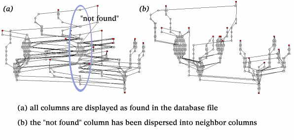 Sort Columns:
At this stage of the algorithm, each node has been
permanently assigned to a column.
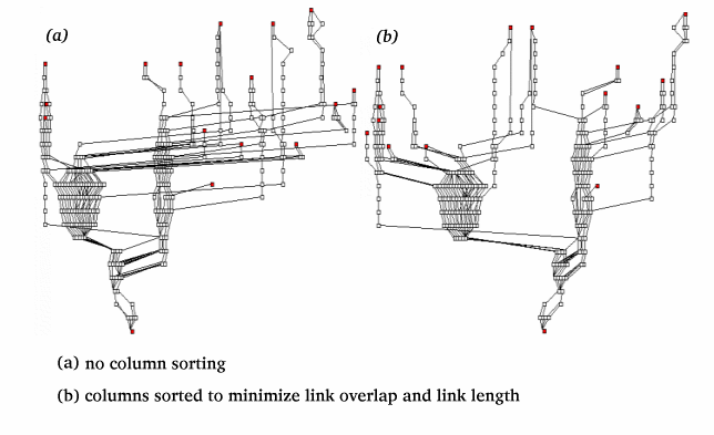
We need to arrange the columns to minimize both the
overlap of links with other columns and the overall
maximum link length.
We implement a greedy algorithm for column
placement which performs a
greedy search of all possible layouts.
To find our optimal placement,
we assign all columns to the "unplaced" set.
This is an unordered set of columns
that contains our pool of placement candidates.
A second set contains all columns that have been placed.
Our algorithm chooses a column from the unplaced set and
tests it in all possible positions relative to columns already placed. For each position, two values are recorded: the number of links that cross the column being placed and its directly adjacent columns (link intersection), and the total length of all the links in the placed set.
Minimization of link intersection takes precedence over minimizing
overall link length in selecting a column placement. Ties in the
column intersection score are broken by using the minimum value for
the total link length score. Once the optimal placement has
been determined, the column is classified as placed and its order
within the placed set is fixed. When all of the unplaced columns
have been placed, the final column order is used to generate an image of the
data set.
 Space Columns:
At this point, the relative positions of all columns are fixed.
Columns will have varying numbers of nodes and, within a column,
some rows will have more nodes than others. If columns were a fixed
size, some nodes would be crowded together, obscuring the details of their connections, while in other regions nodes would be quite sparse.
To address this problem, we vary the space within each
column. We calculate the width of the widest row within a column
and assign that value to the column. Since the X axis represents
the groups specified in the data file and does not involve a physical
distance metric, spacing between columns can be arbitrary.
We expand columns prior to any adjustment of nodes
within the columns so that position of the columns
in coordinate space remains constant during final node placement.
This maintains the relative positions
of all nodes within the image.
Prevent Vertical Link Overlap:
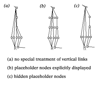 Occasionally our algorithm creates spurious connections
or obscures true connections
between links within a column (see (a) on the right).
This occurs when paths from multiple nodes in a row
converge on a single upstream node.
To prevent vertical overlap, we generate invisible
"placeholder nodes" to reserve space within rows that are spanned by the
vertical link.
Assign Initial X and Y Coordinates to Nodes:
Once horizontal spacing has been determined,
we can assign initial X and Y coordinates for each node
based upon its column number, the column spacing, and its row number within the column.
These values are scaled to screen coordinates for each node.
Coordinate assignment is performed before final node placement so that the X coordinate can be used for sorting nodes within a column.
Arrange Nodes Horizontally:
 We previously reduced the number of tangled paths between nodes
through arrangement of the columns and by allocating sufficient
space in rows with placeholder nodes.
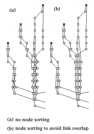
Despite these measures, links within a single
column can overlap repeatedly, producing a tangled graph. By calculating an optimal horizontal arrangement for the nodes, we ensure maximum legibility in the final image.
The algorithm proceeds from the bottom of the image to the top of the image.
Once a node is placed based upon nodes below, it cannot be
moved by future iterations of the algorithm. For each row of a
column in the graph, nodes within the row are ordered by the mean
value of the x-coordinate of their parents (nodes below that link
to them).
In the event that
two nodes in the same row have a parent in common, nodes are
ordered by the mean value of their children (nodes above to which
they link). In children, the algorithm only detects links outside
of the current column since all nodes in the unspread column above the current level have
the same x-coordinate. If a search at a depth of 1 does not break
the tie, we repeat the iterative evaluation of mean x-values first
below, then above each higher (child) node until one of three conditions is met: the tie is broken,
the graph has no more nodes at the given depth, or we have reached the preset maximum depth. If the tie
cannot be broken, the nodes are positioned randomly and the
algorithm progresses to the next higher level.
Thus nodes that are pushed to the left in a column will tend to have their
children above pushed to the left as well. This allows the viewer
to grasp relationships between nodes more easily.
Example (a) shows the results after application of the algorithm to
the tangled graph in (b).
Examples
Actual Otter Examples: (requires java)
Java Documentation
You can find javadoc documentation here. This comprises a detailed description of the java implementation.
Source Code
Source code with sample scripts and input files. plotpaths.tar.gz.
Authors
Project Design:
- John Gallagher
- Bradley Huffaker
- John Gallagher
Acknowledgments:
This material is based upon work supported by the National Science Foundation under Grant No. 9996248 and Grant No. 9711092.
Please send any comments/suggestions you may have to info@caida.org.
