

skping
Background
skping is a standalone RTT and packet loss measurement tool. It is much like ping, but adds plotting and analysis functionality in real time. It can also record data for later analysis.Striving for accurate measurements (contending with sources of error)
RTT and packet loss measurements are nearly trivial to implement using ICMP on our platforms of choice (which are all flavors of UNIX). However, it is not trivial to get accurate data on a typical UNIX operating system. The difficulty lies in accurate timestamping of transmission and reception of measurement packets. The desired measurement in our case is wire time, without the time spent in software on the measurement platform. Software in this context means both measurement software (in user space) and operating system software (in kernel space). The most portable means of timestamping will make a system call to retrieve a timestamp before making another system call to transmit the measurement packet. And in the typical case, there is additional user code between timestamping and transmission (checksum computation, for example). During the system call to transmit, several queueing and other activities take place in the operating system kernel and drivers, and finally the packet is put on the wire. The same things happen in reverse for reception, with the user program getting the packet only after it has passed up through drivers and the IP stack and to the applicaton, at which point it can timestamp.In addition to the issues with the amount of code that must be exercised between user space and the wire, a significant issue on UNIX and other platforms is that of scheduling. CPU cycles are spent across multiple processes, typically using a priority-based time-sharing scheduling policy. Some UNIX platforms offer other scheduling policies, including those outlined in POSIX.4 (now called POSIX 1003.1b-1993). To date, support for real-time scheduling on general purpose UNIX platforms has been spotty.
In my experience, the effects of the typical UNIX scheduler play a far more significant role than IP stack and driver code paths (including queueing). To an extent, my experience also makes perfect sense in a typical UNIX implementation; there are many more things to cause a context switch out of user space than out of kernel space, and those additional things are typically fairly long context switches (higher priority process switched in, etc.)
There are numerous solutions to the timestamping issue. All of them involve work inside the kernel or driver. In my experience, the difference between working in the driver and higher up in the kernel (somewhere in the IP stack) is insignificant compared to the difference between working in the kernel and working in user space. In other words, any type of kernel facility for more accurate timestamping is generally a big win, because it greatly reduces the probability of long or multiple context switches between timestamping and transmission (when sending a packet) and reception and timestamping (when receiving a packet).
One typical solution is to use a packet sniffing facility in the UNIX kernel, for example BPF (Berkeley Packet Filter). Other solutions may involve using the auxiliary data in calls to sendmsg() and recvmsg() (the SO_TIMESTAMP socket option in recent BSD systems, for example).
A second set of solutions may put timestamps in the measurement packet payloads. This is a preferable solution when the measurement application is already maintaining considerable state (for example, a large network management system). While this is not a design constraint for skping (which maintains little state), it was for skitter.
Hence we chose to implement a solution that places timestamps in the payload of the measurement packets, from kernel space. Like SO_TIMESTAMP, it is implemented as a socket option, but only for raw ICMP sockets (
socket(AF_INET,SOCK_RAW,IPPROTO_ICMP)). We place a transmission timestamp (microseconds) in each ICMP echo request sent via a socket with our socket option enabled, and place a reception timestamp (microseconds) in each ICMP echo reply received via a socket with our socket option enabled. This permits each ICMP echo reply to be treated as a self-contained data sample, without any auxiliary state information. The ICMP echo reply contains both the original ICMP echo request transmission timestamp and the reception timestamp.Our implementation is currently based on FreeBSD. It would not be difficult to port to other BSD-derived IP implementations. Our kernel work is done at the IP layer and not in the NIC drivers, so our solution works for any network interface.
Data analysisMost of the data analysis performed by the skping GUI is simple. Order statistics (percentiles) and min/max RTT values are used to display RTT trends. Packet loss is a simple measure of lost packets divided by packets sent. The only reasonably complex data analysis performed by skping at this time is spectral analysis. We use the Lomb periodogram for spectral analysis, mostly due to its ability to handle input samples that are not evenly spaced in time. This is a fairly expensive operation in our current implementation, and hence is only performed over the last N points (which may not exceed 3200). However, frequency analysis has yielded some interesting results for some measurements. More importantly, I believe that signal processing techniques can be applied to RTT (and other) data and reveal problems not necessarily easy to identify via other simple techniques.
Data presentationThere is nothing revolutionary about the data presentation used by skping. In fact, I consider the GUI mundane. However, it has been tuned over a fairly lengthy period of internal use, and is largely driven by simplicity. We are not dealing with complex data, and we are motivated to provide clear presentations without significant user interaction.It is important to understand the context in which skping is normally used. For the most part, it is used in the same context as ping: the user wants to measure in real-time, right now. Hence the default visible plot in the user interface is the Live plot, which shows raw data in real time.
However, the user may also want longer-term historical information, which may be difficult to view in its entirety in raw form. Hence we use a candle plot combined with a bar chart to store historical RTT data (max, min, median, 25th percentile, 75th percentile) and packet loss. We call this the History plot. Like the Live plot, it is a rolling plot (it does not save data indefinitely, but instead rolls old data off the left edge of the plot).
We also provide a simple RTT Distribution plot. This is a histogram with RTT on the x-axis (divided into 50 intervals of equal time), the number of hits in each RTT interval on the y axis (shown as blue bars), and a vertical green bar representing the median.
Finally, we provide a plot of a Lomb periodogram of the last N input points. The plot itself isn't very interesting, but frequency analysis applied to RTT data can occasionally yield interesting results.
The skping user interface
The user interface for skping displays several plots of the RTT and packet loss data in real time. It also permits printing of the plots (PostScript, JPEG or PNG output). Finally, a few plot parameters can be changed from within the GUI.The plots and some other parts of the user interface are implemented using XRT/PDS from KL Group. CAIDA currently owns an XRT/PDS license for Sparc/Solaris and another for Linux. XRT/PDS is not available for FreeBSD, so the GUI is actually a separate program from skping, which permits us to use the GUI program under Linux emulation on FreeBSD while using a native FreeBSD version of skping (with kernel timestamping).
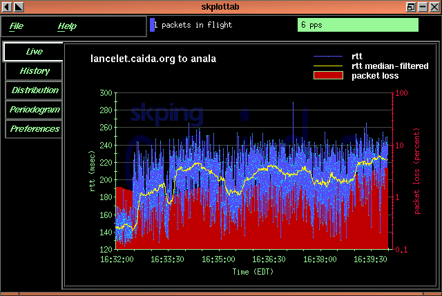
Live plot
The Live plot shows the raw RTT measurements, median-filtered RTT measurements and windowed packet loss. The raw RTT measurements are cyan points connected by blue lines. The median-filtered RTT measurements are yellow. The packet loss is a red area behind the RTT data, and the y-axis for the packet loss (red y-axis on the right side) is logarithmic.The data shown here was for a particularly bad day of connectivity from CAIDA Ann Arbor to CAIDA San Diego. The Live plot below is a screenshot of skping running in real time, with 3200 points on the x-axis and the median window (for drawing the yellow median-filtered line) was set to 50 points.
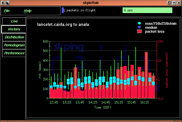
History plot
The History plot shows historical RTT and packet loss. The RTT data is shown with a candle plot. The top of the green candle line is the maximum RTT. The top of the cyan box of the candle is the 75th percentile RTT value. The bottom of the cyan box is the 25th percentile RTT value. The horizontal blue line is the median RTT value. The bottom of the candle line is the minimum RTT value. The packet loss is represented as a red bar behind the RTT candle. The scale for the packet loss is logarithmic, as indicated on the red y axis on the right side of the plot.Distribution plot
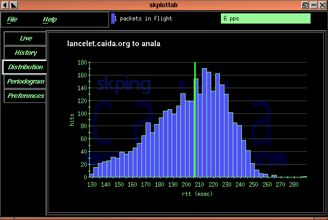
The Distribution plot shows the distribution of RTT measurements over the last N points (where N can be set in the Preferences). The blue bars show the distribution and the vertical green line represents the median.Periodic signal in Live plot
Significant periodicity in RTT data on the Internet is rare. However, it's not quite as difficult to find as the proverbial needle in a haystack. In fact in my experience, it's not even close to "Look hard enough, find anything." Here's an example from the day I created this page (October 29, 1999). This is the Live plot, and the RTT data (blue) seems to have periodic content:Periodogram plot
Sure enough, spectral analysis indicates a fairly strong periodic signal around .41 Hz (a period of roughly 2.4 seconds):Periodic signal in another Live plot
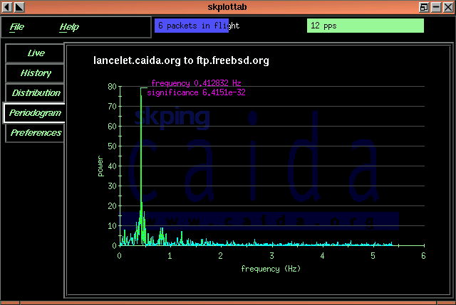
One of the many reasons this is interesting: this behavior would not be observed at a sampling rate less than once every 1.2 seconds (Nyquist sampling theorem). This has implications for measurement software, in the sense that sampling at lower rates may conceal behavior whose identification may be fruitful.
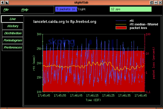
Obviously, the cause of the periodicity in our example (and others) is of great interest. In our example, I suspect global TCP synchronization (ftp.freebsd.org is actually ftp.cdrom.com, purported to be the busiest FTP server on the Internet). It would be interesting to identify the bottleneck queue (I'll try on November 1st) and see if we can coerce someone into enabling RED on that queue (I'm assuming it's not enabled).
Periodogram plotHere's another example, and it hits close to home. This data was observed on October 30, 1999 for lancelet.caida.org (in my home in Ann Arbor, Michigan) to anala.caida.org (in San Diego, California). The Live plot was set to hold 3200 points (the Points setting in Preferences), and the median filter was set to 10 points. skping is receiving 24 packets per second.
Yikes. That's what I'd call a periodic signal.Modifying preferences
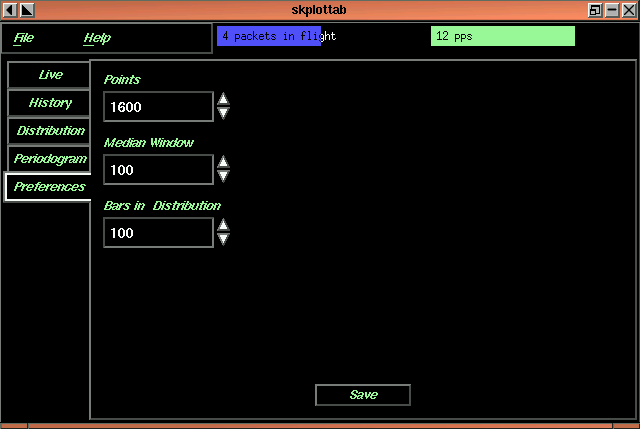
The Preferences screen may be used to change a few of the parameters used for the plots. You may also save your preferences from this screen, which will cause them to be used the next time you start skping.The Points setting affects all of the plots. It determines the maximum number of raw RTT measurements kept in memory. The Live plot will contain (at most) this number of points. Each History plot candle will represent this number of points. The Distribution plot will contain this number of points. The Periodogram plot will be constructed from this number of points.
The Median Window setting determines the number of points used to compute the median line (yellow) in the Live plot. A high setting will cause smoothing of the median linew, while a low setting will cause the median to more closely follow the raw data.
The Bars in Distribution setting determines the number of bars (intervals) in the Distribution plot.
The Save button saves your current preferences. This will cause your current preferences to be used the next time you start skping.
Recording data
You may record data with skping by using the -r recordfile command line option when you start skping. The data is stored as arts++ RTT time series data. You may also use the -X command line option when recording data. This will disable the GUI, which allows you to record data without an X session.
Examining recorded data
I am still working on tools for examining recorded data, including text reporting and graphical plotting tools. There are some things that can be done with recorded data and offline processing that are not easily done in real time (signal processing over long time periods with high sampling frequency, long normalization periods, etc.). I hope to incorporate more elaborate analysis and long-range analysis in these tools.
Further research areas
While RTT measurements for a single (source, destination) pair yield a simple dataset and have been studied for many years, it is still my belief that there are interesting behaviors to be observed on several time scales that are not identified by typical tools. I think it is important to examine signal processing techniques that can be applied to time series data like RTT measurements to yield more useful information. In my first example of periodicity above, the packet loss on the bottleneck queue is likely well known, since it is easily observed via simple active measurements like our own as well as SNMP queries for dropped packet counters (in this case we suspect congestion and hence ifOutDiscards on the bottleneck link would likely tell us that we're dropping packets). However, it is unlikely that these typical simple measurements would identify the periodic behavior we have observed. This is unfortunate, because it is also likely that enabling RED on the bottleneck queue would significantly improve the behavior of the bottleneck queue.
Daniel W. McRobb
Copyright © October 1999 CAIDA