Internet topology at router- and AS-levels, and the dual router+ASInternet topology generator
Overview of the topology generation process
The main idea behind our dual Internet topology generator is to rescale a measured Internet topology to a given target size preserving some basic statistical characteristics of the measured topology. Specifically, we first rescale the measured AS topology to any given target size using methods from the paper "Graph Annotations in Modeling Complex Network Topologies", and then populate each AS with a router topology generated from scratch using methods from the paper "Hyperbolic Geometry of Complex Networks" matching some average properties of per-AS router topologies. The details of this program are outlined below.
Internet topology datasets and their pre-processing
The input to our topology generator process is a measured "dual-graph" of the Internet, consisting of the router-level topology, the AS-level topology overlaid on top of the router-level topology, and the annotation for each router indicating which AS the router belongs to. We take this data from CAIDA's Internet Topology Data Kit (ITDK). The ITDK provides the Internet router-level graph, from which we extract the AS topology via mapping each IP interface to an AS using prefix-to-AS mapping. The ITDK also provides router-to-AS assignments, indicating which AS owns each router. To construct the AS overlay from the router-level graph, we use CAIDA's BGP-derived AS-relationship dataset, which gives us the type of relationship between each pair of ASes.
We first prune the router graph from ITDK 2010-07 as follows:
- We remove all routers of degree 1 from the router-level graph. We do not do this process recursively, i.e., the resulting graph is not the 1-core.
- We use the router assignment dataset, which indicates which AS each router was assigned to.
- We restrict the set of ASes in our measured graph to the set of ASes that had at least one router assigned to them in the pruned graph, i.e., only those ASes that were seen in the ITDK. We obtain the relationships between these ASes from the CAIDA AS relationship data.
- We then annotate each AS with the following measured statistics of that AS: The number of customers, number of providers, number of peers, and number of routers.
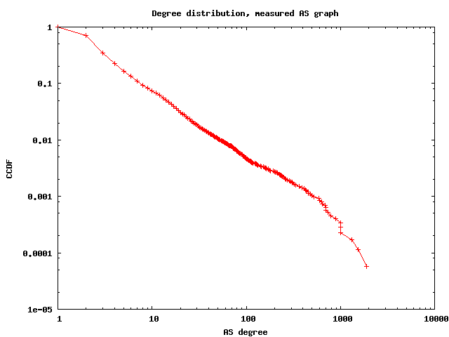
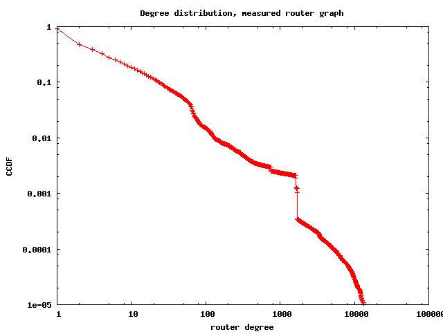
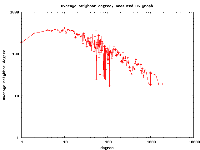
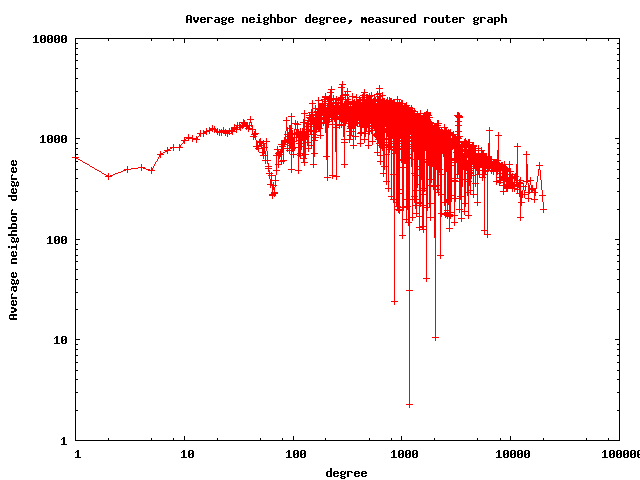
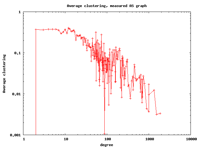
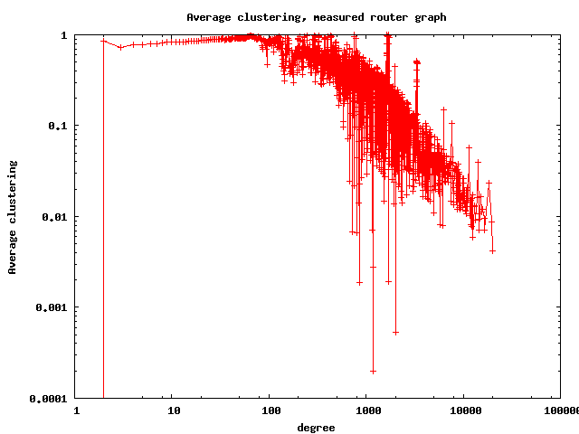
The resulting router graph has 1,204,038 nodes (routers), 13,349,748 links, its average degree is 22.17, average clustering 0.73, and the best fit for the power law exponent of the degree distribution is 2.34. The AS graph has 17492 ASes, 47804 links, average degree 5.4, average clustering 0.25, and the best fit for the power law of the degree distribution is 2.13. Below we also show few other basic topological properties of these graphs: the degree distribution, average degree of neighbors, and degree-dependent clustering.
Rescaling
We briefly describe the process we use to rescale the dual router+AS graph. We separate the process of rescaling the AS-level and router-level topologies as follows:
- We extract the distributions of the number of customers, providers, peers, and number of routers per AS (called annotation distributions) in the ITDK-measured AS graph, and fit these distributions with smoothing splines.
- The annotation distributions do not tell us anything about the correlations among annotated degrees of the same node, i.e., how many customers, providers, and, simultaneously, peers a specific AS has. These correlations are present in the Internet. We extract the copula of the annotated degree distribution, which gives us the correlation structure between the number of customers, providers, peers, and routers of an AS.
- If N is the number of ASes required in the rescaled graph, we generate N samples from the annotation distributions of the number of customers, providers, peers and routers. We use the copula of the annotated degree distribution to produce ASes in the rescaled graph with certain number of customers, providers, peers, and routers.
- We use the procedure described in the paper "Graph Annotations in Modeling Complex Network Topologies" to construct the graph at the AS-level. This procedure takes as input a set of N ASes, and the annotated degree distribution of the number of customers, providers, peers, and routers of each AS.
- We then generate an internal router-level topology for each AS in the rescaled graph as described below.
- For each AS-level link between ASes X and Y, we randomly choose routers in AS X and AS Y, and connect them with a router-level link.
Generating a router graph for each AS
In the previous step, we rescaled the graph at the AS-level, creating a collection of N ASes, each with a given number of routers. The next step is to to connect the routers that belong to each AS into a router-level topology for that AS.
To simplify the automatic router-level topology generation process, we use the topology generator from the paper "Hyperbolic Geometry of Complex Networks". This generator produces random graphs with any given target values of graph size, average degree, average clustering, and power-law exponent of the degree distribution. Therefore we are interested in how widely these characteristics vary from the router graph in one AS to another, and how close these graphs to their corresponding random graphs.
For this end we analyze the router-level graphs of a set of 400ASes. We first isolate the router-level topologies of these 400 ASes using the router-level graph and AS assignment information from ITDK, and then measure their statistical characteristics above. We also check how these characteristics depend on the graph size.
From the results presented in the next section we find that the distributions of these characteristics across the considered 400 ASes are not too wide, indicating that according to these characteristics, router topologies of different ASes are roughly similar. Therefore for simplicity we fix the values of the average degree, clustering, and power-law exponents in the hyperbolic generator to their median values in the corresponding distributions.
To test how close real router graphs are to their random counterparts with the same degree distribution and average clustering, we randomly rewire the real graphs preserving these two properties. The details are in the last section. The results presented there exhibit one common trend: clustering of low-degree nodes in real graphs is noticeably higher than in their randomizations, which is expected. Unfortunately we cannot preserve this high-clustering of low-degree routers without trading off generator simplicity. There are no other systematic differences between real and random graphs, so that we fix the value of average clustering in the hyperbolic router generator to the median value of average clustering observed in the real router graphs.
The distributions of the average degree, clustering, and power-law exponents in router topologies of 400 ASes
Average degree
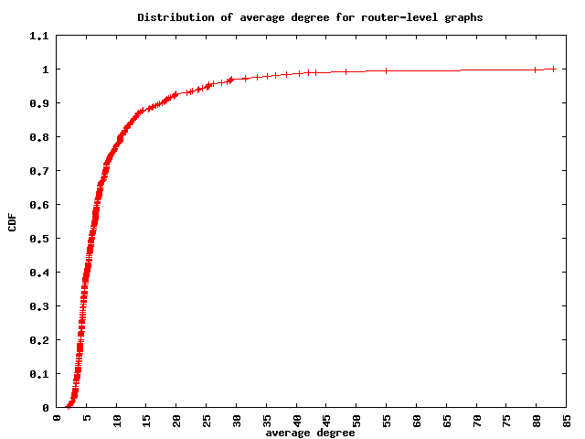
The figure below shows the CDF of the average degree calculated for each graph. We find that the median average router degree for these ASes is 5.
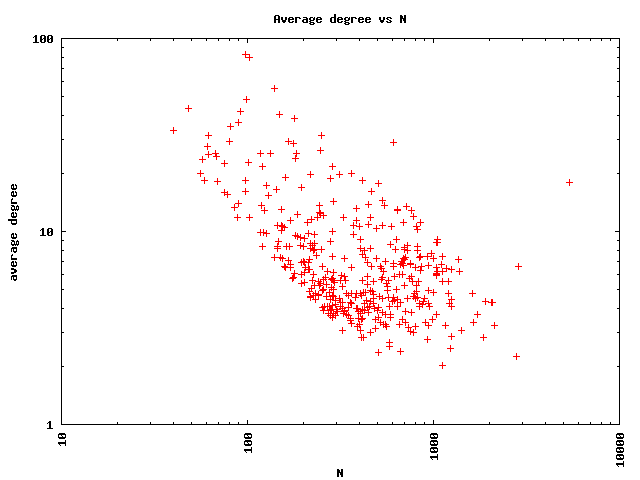
Next, we see how the average degree in the router-level graph of an AS depends on the number of routers of that AS (size of that AS). We find an overall decreasing trend of the average degree as the size of the AS increases. This, however, is due to the set of ASes we have chosen for this analysis. We chose 400 ASes for which the router-level graphs have between 1000 and 5000 links (so that they can be analyzed in a reasonable amount of time). These graphs, however, have variable number of routers, and approximately similar number of links. This causes the scatter plot to show a decreasing trend of the average degree as a function of the number of routers in the AS.
Average clustering
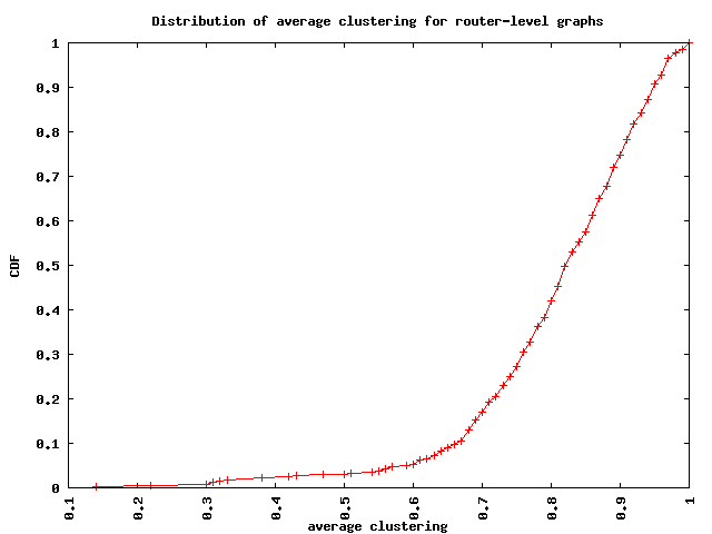
The figure below shows the CDF of the average clustering calculated for each graph. We find that the median average clustering for these ASes is 0.8.
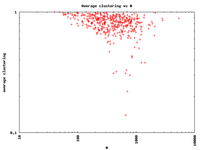
We also look at how the average clustering of the router-level graph of an AS depends on the size of that AS in terms of the number of routers. There is no noticeable trend in the average clustering as a function of the size of an AS.
Power-law exponents
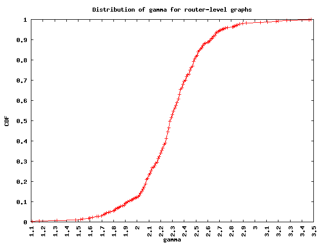
The figure below shows the CDF of the degree distribution power-law exponents calculated for each graph. We find that the median gamma for these ASes is 2.3.
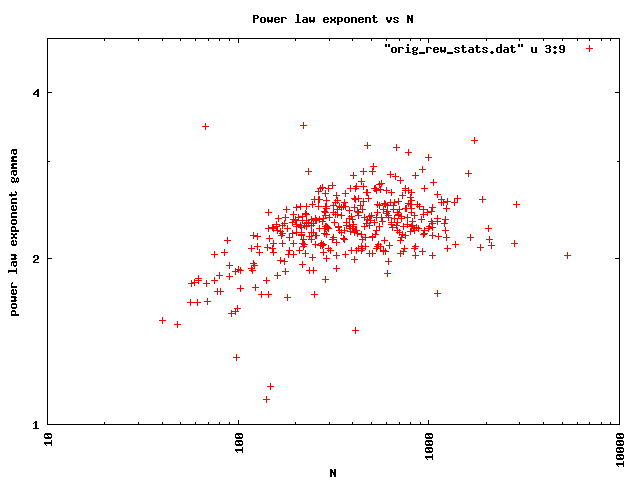
We also look at how the exponent of the power-law degree distribution depends on the size of the router-level graph of an AS in terms of the number of routers. We find a generally increasing trend of the power law exponent with the size of the AS.
Random rewiring that preserves the degree distribution and average clustering in router graphs
This randomizing rewiring procedure is as follows:
- Pick two edges v1-v2 and v3-v4. Check that edges v1-v4 and v2-v3 do not already exist.
- Count the number of triangles these edges were involved in before rewiring: for each node v5 which is a neighbor of v1, if the edge v2-v5 exists, then increment the number of triangles; and for each node v6 which is a neighbor of v3, if the edge v4-v6 exists, then increment the number of triangles. Let n_ini be the number of triangles computed this way, before the rewiring attempt.
- Rewire edge v1-v2 to v1-v4 and edge v3-v4 to v2-v3. This rewiring trivially preserves the degree distribution.
- Count the number of triangles after the rewiring: for each node v5 which is a neighbor of v1, if the edge v4-v5 exists, then increment the number of triangles; and for each node v6 which is a neighbor of v2, if the edge v3-v6 exists, then increment the number of triangles. Let n_aft be the number of triangles computed this way, after the rewiring attempt.
- If n_ini == n_aft, then keep the rewired graph, else revert to the set of original edges v1-v2 and v3-v4.
- Repeat this procedure until we achieve the target number of rewirings (10000), or the maximum number of attempted rewirings (1000000) has been reached.
For each AS, we then compute the average neighbor node degree ANND(k) and average clustering C(k) of nodes of degree k for the original and rewired graphs for each of the 400 ASes in our study. Please refer to the statistics of the original and randomized graphs for each of the 400 ASes.
Additional Content
Internet topology at router- and AS-levels, and the dual router+ASInternet topology generator
This page is supplementary material for the design of our dual router+AS level topology generator.
