Universal Laws of Structural Dynamics of Large Scale Graphs - Proposal

The original proposal is shown below. For the PDF version of the proposal for "DARPA grant HR0011-12-1-0012: Universal Laws of Structural Dynamics of Large Scale Graphs", please see the proposal in PDF.

1 Innovative Claims

The main long-term goals that motivate this project are the detection of anomalies in the dynamics of large graphs representing real networks (complex networks in short), as well as the prediction and control of their behavior.

The most widely used approaches to these problems are based on data mining, machine learning, and statistics, yet their limitations are well known. These approaches are often highly tailored to a specific network or specific task, leading to overfitting, overtraining a method on a specific dataset, and thus diminishing the predictive power of the method and its overall efficiency. Worse yet, extreme manual care and special expertise are routinely required to tune these approaches for a task at hand, rendering them nearly impossible to use in everyday practice with constantly changing requirements and conditions.

We strive to develop a radically different approach. Our goal is to discover the universal laws governing the dynamics of complex networks. The main impact and practical significance of the proposed work is the knowledge of such laws that will allow us to predict network dynamics, while abnormal dynamics deviating from such laws will then signify anomalous activity in the network.

Our recent work yields strong indications that such laws exist. We developed a powerful and unique geometric theory explaining the ubiquitous common structure of complex networks, and linking this structure to the optimality of their common functions. The core building block of this theory is hyperbolic geometry. We have shown that random geometric graphs built on top of Riemannian manifolds with negative curvature exhibit structural properties common to many real networks.

The main limitation of the theory developed so far is that from the mathematical perspective, it rigorously applies only to static graphs. To detect anomalies, to predict network behavior, we need a mathematically rigorous theory for dynamic graphs that grow and evolve.

In this project, we propose to make the first step towards developing such a theory by mapping our hyperbolic model of complex networks to pseudo-Riemannian geometry. Pseudo-Riemannian geometry is the geometry of manifolds, in which one coordinate can be associated with time, making this geometry a perfect candidate to model dynamic graphs evolving in time, and to search for the universal laws of their dynamics.

Succinctly, we have shown that random geometric graphs on hyperbolic Riemannian manifolds model adequately the structural properties of large real networks. The main premise that we set to prove during the first year of this project is that random geometric graphs on certain pseudo-Riemannian manifolds also model the dynamical properties of these networks.

If our first-year tasks are successfully completed, then in subsequent years we will propose to: (i) identify the equations describing the dynamics of random geometric graphs in the resulting model; (ii) develop a set of tools and methods, based on these equations, to predict network dynamics and detect anomalies; and (iii) apply the developed methods to real networks.

2 Technical Rationale and Approach

Many different real networks exhibit certain structural similarities [1], suggesting that there is a possible universal explanation for their common structure. In our recent work [2,3,4,5,6,7,8] we have found a mathematically satisfactory explanation for this phenomenon. Specifically, we have defined and studied random geometric graphs in hyperbolic spaces. The intuitive motivation to employ hyperbolic geometry is that large networks frequently exhibit hierarchical tree-like organization, and hyperbolic geometry is the geometry of tree-like spaces. This intuition finds mathematically rigorous formalization in a series of seminal works by Gromov [9]. In the simplest case, we define random hyperbolic graphs (RHGs) by the following construction: 1) distribute uniformly at random a set of nodes over a compact patch (e.g., the compactification of an open ball) in a hyperbolic space, and 2) connect each pair of points iff the distance between them is less than the ball radius. In other words, the connectivity in RHGs is defined by intersections of balls, which form a base of the manifold topology. We have proved that RHGs possess the most common structural properties of many real networks: (a) strong clustering, i.e., high probability of connections between two neighbors of the same node; and (b) heterogeneous distributions P(k) of node degrees k, which often follow power laws P(k) ∼ k^−γ. Leaving the detailed discussion of the strengths of this approach to Section 4, here we note its two main limitations: 1) RHGs form an ensemble of intrinsically static graphs, while real networks are dynamic, and 2) the power-law exponent in RHGs is γ = 3, while in real networks, γ is never 3 but often close to 2 [1]. The model admit adjustments yielding graphs with γ = 2 if one chooses to distribute nodes in the space non-uniformly. In this case however, RHGs are no longer random geometric graphs and, therefore, they can no longer be formally considered as discretizations of smooth hyperbolic manifolds. Therefore the hope to derive, in a mathematically rigorous way, the universal laws describing the structure and dynamics of real networks using hyperbolic Riemannian manifolds should be abandoned. Yet the observations above suggest that real networks can be described by somewhat similar geometric spaces or manifolds. Here we set to find such spaces in the category of pseudo-Riemannian manifolds.

Pseudo-Riemannian manifolds are manifolds with non-degenerate metric tensors (vs. positive-definite tensors in Riemannian manifolds), meaning that distances between two different points on the manifold can be positive, negative, or zero. If the metric tensor has signature (−,+,+,…,+), then the manifold is called Lorentzian. Lorentzian manifolds form an important and well-studied class of pseudo-Riemannian manifolds [10]. In these manifolds, the coordinate corresponding to the minus sign in the signature represents time. For each point p on the manifold, one can split the set of all points at negative (timelike) distances from p into two parts: I⁻(p)-all points in the past of p whose time coordinate is smaller than p's, and I⁺(p)-all points to the future of p. If point q ∈ I⁺(p), then intersection I⁻(q)∩I⁺(p) is called an Alexandrov set. These sets form a base of the manifold topology for a wide class of manifolds [11], including all the manifolds that we will consider in this project. That is, Alexandrov sets are analogs of open balls in the Riemannian case. This observation instructs us to define random Lorentzian graphs (RLGs) as follows: 1) distribute uniformly at random a set of nodes over a compact patch in a Lorentzian manifold, and 2) connect each pair of points iff the distance between them is negative.

The rationale to focus on Lorentzian manifolds is two-fold: 1) these manifolds are similar to hyperbolic manifolds in two key aspects: a) exponential expansion of space, and b) symmetry properties; but they are also different in two other key aspects: a) explicit inclusion of time, and b) metric differences yielding γ = 2 in RLGs instead of γ = 3 in RHGs. To elaborate, the exponential dependency of the volume of balls on their radii in hyperbolic geometry is the key metric property responsible for the emergence of heterogeneous power-law degree distributions in RHGs, common to many real networks. The same property characterizes certain Lorentzian manifolds-in particular, the manifolds with constant positive or negative curvature, known as de Sitter and anti-de Sitter spaces. The symmetry groups of these spaces, i.e., the groups of their isometries, are SO(1,d) and SO(2,d−1), where d is the space dimension. The former group is the same as the isometry group of the hyperbolic space. A wider class of spherically symmetric spaces are invariant with respect to SO(d), a subgroup of SO(1,d). Yet Lorentzian manifolds are different from hyperbolic spaces in that they explicitly model time, so that in contrast to RHGs, RLGs are intrinsically dynamic graphs. Finally, the space expands exponentially in Lorentzian manifolds with an exponent different from that in the hyperbolic space, yielding γ = 2 in RLGs, vs. γ = 3 in RHGs (Section 4).

In summary, Lorentzian manifolds possess the key desirable properties of hyperbolic manifolds, but favorably differ from them exactly where the latter fail short to describe rigorously the reality of large networks. Collectively, these considerations dictate the following first step on our agenda: identify a spherically symmetric Lorentzian manifold M dual to the hyperbolic space H in the sense that there exists an invertable map Φ from M to H that sends Alexandrov sets in M to intersections of balls in H.

3 Statement of Work

distribute uniformly at random a set of nodes over a compact patch (e.g., the compactification of an open ball) in a hyperbolic space, and
connect each pair of points iff the distance between them is less than the ball radius.

In other words, the connectivity in RHGs is defined by intersections of balls, which form a base of the manifold topology. We have proved that RHGs possess the most common structural properties of many real networks-strong clustering, i.e., high probability of connections between two neighbors of the same node, and heterogeneous distributions P(k) of node degrees k, which often follow power laws P(k) ∼ k^−γ. Leaving the detailed discussion of the strengths of this approach to Section 4, here we note its two main limitations:

RHGs form an ensemble of intrinsically static graphs, while real networks are dynamic,
the power-law exponent in RHGs is γ = 3, while in real networks, γ is never 3 but often close to 2 [1].

The model admit adjustments yielding graphs with γ = 2 if one chooses to distribute nodes in the space non-uniformly. In this case however, RHGs are no longer random geometric graphs and, therefore, they can no longer be formally considered as discretizations of smooth hyperbolic manifolds. Therefore the hope to derive, in a mathematically rigorous way, the universal laws describing the structure and dynamics of real networks using hyperbolic Riemannian manifolds should be abandoned. Yet the observations above suggest that real networks can be described by somewhat similar geometric spaces or manifolds. Here we set to find such spaces in the category of pseudo-Riemannian manifolds.

distribute uniformly at random a set of nodes over a compact patch in a Lorentzian manifold, and
connect each pair of points iff the distance between them is negative.

The rationale to focus on Lorentzian manifolds is two-fold:

these manifolds are similar to hyperbolic manifolds in two key aspects:
1. exponential expansion of space, and
2. symmetry properties;
but they are also different in two other key aspects
1. explicit inclusion of time, and
2. metric differences yielding γ = 2 in RLGs instead of γ = 3 in RHGs.

To elaborate, the exponential dependency of the volume of balls on their radii in hyperbolic geometry is the key metric property responsible for the emergence of heterogeneous power-law degree distributions in RHGs, common to many real networks. The same property characterizes certain Lorentzian manifolds-in particular, the manifolds with constant positive or negative curvature, known as de Sitter and anti-de Sitter spaces. The symmetry groups of these spaces, i.e., the groups of their isometries, are SO(1,d) and SO(2,d−1), where d is the space dimension. The former group is the same as the isometry group of the hyperbolic space. A wider class of spherically symmetric spaces are invariant with respect to SO(d), a subgroup of SO(1,d). Yet Lorentzian manifolds are different from hyperbolic spaces in that they explicitly model time, so that in contrast to RHGs, RLGs are intrinsically dynamic graphs. Finally, the space expands exponentially in Lorentzian manifolds with an exponent different from that in the hyperbolic space, yielding γ = 2 in RLGs, vs. γ = 3 in RHGs (Section 4).

Lorentzian manifolds thus possess the key desirable properties of hyperbolic manifolds, but favorably differ from them exactly where the latter fail short to describe rigorously the reality of large networks. Collectively, these considerations dictate the following first step on our agenda: identify a spherically symmetric Lorentzian manifold M dual to the hyperbolic space H in the sense that there exists an invertable map Φ from M to H that sends Alexandrov sets in M to intersections of balls in H. Specifically, our tasks are:

Find a Lorentzian manifold M such that there exist bijection Φ between M and hyperbolic space H that preserves the volume form, and maps Alexandrov sets in M to intersections of balls in H.
This is the most involved task, consisting of many subtasks:
1. Prepare a candidate list of manifolds M. The simplest Lorentzian manifolds will be considered first, such as the manifolds with constant negative, zero, or positive curvature, but more complicated manifolds may also have to be considered, e.g., homogeneous and isotropic manifolds, or manifolds with only spherical symmetry. Then, for each M in the list:
2. Introduce a coordinate system on M. The choice of the coordinate system will be dictated by the group of isometries of M. Since the candidate spaces are expected to be at least spherically symmetric, the most natural choice for the coordinate system is the spherical foliation of M, (t,Ω), where t is the time coordinate and Ω is the vector of angular coordinates on the sphere. The corresponding coordinate system on H is the standard spherical coordinate system (r,Ω), where r is the radial coordinate. Therefore due to these symmetry considerations, we expect that Φ(t,Ω)=(f(t),Ω), so that the next step is:
3. Find function r=f(t) yielding Φ with the required properties. Mathematically, these properties (volume-form preservation and mapping Alexandrov sets to ball intersections) translate to a system of equations that function f(t) must satisfy. This system might not have a solution, meaning that Φ does not exist for a given M. If a solution exists, then we have a proof for the existence of the required bijection Φ for M, in which case we will also have to:
4. Prove that Φ is invariant under the group of isometries of M and H. This proof is important, because if Φ is not invariant, then it may be an artifact of a particular choice of the coordinate system above.
Derive the structural properties of random geometric graphs in M.
In contrast to random geometric graphs in H, we do not have much freedom in defining random geometric graphs in M. The only possible definition is to select a compact patch in M, e.g., lying between t=0 and t=τ, where τ > 0 is a parameter, and distribute nodes uniformly at random, e.g., via the Poisson point process, over this patch. To respect the Alexandrov topology on M, we then have no choice other than connecting all node pairs located at negative distances. We will then use the standard tools in differential geometry to compute the volumes of the patch and Alexandrov sets in it, to derive analytically the basic structural properties of these graphs, such as their size, average degree, degree distribution, clustering, etc.
Derive the dynamical properties of graphs in Task 2.
The random graphs from Task 2 are intrinsically dynamic as soon as τ is not a constant but a variable that models graph growth with time. We will use the same methods as in Task 2 to describe analytically the dynamic process of the evolution of the graph structure with time τ.
Validate the analytic results in Tasks 2-3 in numeric experiments:
1. Implement the graph model from Tasks 2-3 in software, and
2. Simulate these random graphs, computing their structural and dynamical properties, and comparing these properties with the theoretical results in Tasks 2-3.
Apply the results in Tasks 2-4 to real-world network data:
1. Collect real network data. We will obtain detailed historical data on networks that evolve in time, vs. their one-time snapshots. We have good experience working with the Internet data, as well as with Pretty-Good-Privacy data on the social network of trust relations between people. Other evolving network data may be also considered.
2. Process the data. We will post-process the raw collected data, and extract from it the structural and dynamical graph properties studied in Tasks 2-4.
3. Apply the theoretical results to the real data. Finally, we will investigate how accurately the theoretical and numerical results in Tasks 2-4 describe the extracted structural and dynamical properties of the real graphs.

4 Detailed Technical Approach

4.1 The structure and function of large networks

In this project we will rely on the geometric network theory developed in our recent work [2,3,4,5,6,7,8] which we review first. The main motivation for this theory was to establish a precise connection between common structural properties of large networks and their functional efficiency. The intuition driving that research program was that these networks must have their observed common structure not without a reason, and the main reason is likely that this structure optimizes network efficiency with respect to some functions, common to many networks.

Among many functions that different networks perform, information transmission or transport stands out as the most common. It is the main function of the Internet, social networks, the brain, cell regulatory networks-to name just a few examples. In these examples, information transmission is not akin to diffusion. Instead, information is often destined or targeted to specific (groups of) nodes. The Internet is an obvious example, but so is the brain, which would not function well if it were not an efficient information router [12]. Routing is a well-understood computational task if the network topology is globally known to all nodes; much less so otherwise. Nevertheless, many real networks, e.g., neural and social networks, efficiently route information even though their nodes have no knowledge of the global network structure. One plausible explanation assumes the existence of latent geometry underlying the network. If this latent space exists, then even if all that each node knows is only local information about the latent coordinates of its neighbors, it can still route by forwarding information to its neighbor closest to the information target in the latent space. One can introduce several metrics of network navigability, that is, of how efficient this geometric routing process is-how many routing paths reach their targets, how optimal they are, how robust this efficiency is with respect to noise and missing or corrupted information about network structure, etc.

Remarkably, using our geometric approach, we have shown that all these navigability metrics are theoretically the best possible if the network has a structure with properties common to many real large graphs, and if the latent geometry is hyperbolic. The first "if" suggests that the structure and function of large networks are indeed tightly knit. The second "if" underlies our proposed work, to describe which we first outline in more detail the state of the theory we have developed so far.

4.2 Random hyperbolic graphs (RHGs)

Figure 1: Synthetic network generated by the geometric network model described in the text. The number of nodes is N=740, and the radius of the hyperbolic disc is R=15.5, fixing the average degree in the network to ―k=5. The shaded areas show two hyperbolic discs of the radius R centered at the circled nodes located at distances r=10.6 (upper node) and r=5.0 (lower node) from the origin shown by the cross. The shapes of these discs are defined by the expression for the hyperbolic distance in the text, and according to the model, the circled nodes are connected to all the nodes lying within their discs, as indicated by the thick links. In particular, the two circled nodes lie within each other's discs.

Our theory assumes that a latent hyperbolic space underlies a network. Hyperbolic spaces can be informally thought of as "smooth versions" of trees [9], reflecting the hierarchical tree-like organization of complex networks [6]. This latent hyperbolic geometry then shapes the network structure, in the simplest case, according to the following constructive definition of RHGs:

consider a closed disc of radius R in the hyperbolic plane;
distribute N ∼ e^R nodes on it with the uniform node density, e.g., by the Poisson point process; and
connect each pair of nodes if the hyperbolic distance between them is less than R, see Fig. 1.

The analytic derivation of RHGs' structural properties uses the following two facts from hyperbolic geometry:

exponential expansion of space, or formally, the fact that the element of length ds and volume form dV written in polar coordinates (r,θ), where r and θ are the radial and angular coordinates, are

ds²

dr²+sinh²r dθ²,

(1)

sinhr dr dθ,

(2)

from which it follows that the radial density of nodes distributed uniformly over a hyperbolic disc of radius R is

ρ(r)=

sinhr

coshR − 1

≈ e^r−R, where r ∈ [0,R]; and

(3)

the hyperbolic distance x_ij between two points i and j located at polar coordinates (r_i,θ_i) and (r_j,θ_j) is given by

x_ij = arccosh(coshr_i coshr_j − sinhr_i sinhr_j cosθ_ij) ≈ r_i+r_j+2lnsin

θ_ij

(4)

where θ_ij = π− |π− |θ_i − θ_j|| is the angular distance between i and j.

Using these two facts, we proved that random hyperbolic graphs (RHGs) defined above have a heterogeneous distribution P(k) of node degree k-specifically, a power law P(k) ∼ k^−γ with exponent γ = 3-while their clustering, i.e., the number of triangular subgraphs, is the strongest possible for graphs with this degree distribution. The first property is easy to see, and it follows from the exponential expansion of space. Indeed, since the node density in the plane is uniform, the expected degree k(r) of nodes located at radial coordinate r in Fig. 1 is proportional to the area A(r) of the intersection of two discs of the same radius R whose centers are at distance r from each other. We showed that as a consequence of the exponential expansion of space, this area decreases with r exponentially,

A(r) ∼ k(r) ∼ e^[1/2](R−r),

(5)

with exponent 1/2. The combination of two exponentials, the density of nodes in Eq. (3) and their expected degrees in Eq. (5), yields the power-law degree distribution in RHGs with exponent γ = 1+2=3.

The RHG definition can be generalized to any space dimension and any curvature, yielding essentially the same results. One can also introducing network temperature, a parameter controlling the strength of the tie between latent geometry and network topology. Clustering is then a decreasing function of temperature: at zero temperature, clustering is the strongest possible as described above, and it decreases to zero at a certain phase-transition value of temperature. If one forces the node density in the space to be non-uniform, ρ(r) ∼ e^α(r−R) with parameter α ≥ 1/2, then this parameter affects γ via γ = 1+2α. Finally, the tunable constant in the N ∼ e^R scaling controls the average degree in the network. For further details, see [5,6].

We next discuss the strengths and weaknesses of the RHG model:

Strengths. The attractive features of the described network model include:
1. The model has only three parameters-temperature, curvature, and the N vs. R scaling constant-that can be tuned to generate graphs with any given clustering strength, heterogeneous degree distribution, and average degree. Strong clustering and heterogeneity exhaust all commonalities of real large networks. These networks are different from each other in other respects. Therefore the model is an adequate baseline to start studying fundamental laws in the theory of large networks.
2. Clustering and heterogeneity are not "enforced," but appear as natural consequences of the metric property and negative curvature of the underlying hyperbolic geometry.
3. By construction, the modeled networks have a latent space underneath, and we show that strong heterogeneity and clustering, commonly observed in real networks, ensure maximum navigability, thus relating the structure of complex networks to the optimality of their transport functions.
4. In certain limiting parameter regimes, e.g., infinite temperature and/or curvature, the model reduces to well-studied ensembles of random graphs. Specifically, classical (Erdös-Rényi) random graphs, random graphs with a given degree distributions, and random geometric graphs, are all degenerate cases within the model.
Weaknesses. The two significant limitations of the model are:
1. The model is a model of static graphs, while all real network evolve in time. Specifically, the described model belongs to a class of models known as exponential random graphs [13]. These models describe maximum-entropy ensembles of static graphs satisfying certain structural constraints, which are the specified values of the average degree, degree distribution, and clustering in our case. Informally, these graphs can be thought of as "maximally random" static graphs satisfying the structural constraints above.
2. The uniform distribution of nodes in the hyperbolic space yields power-law graphs with exponent γ = 3, never observed in reality-a vast majority of real networks have γ close to 2. The power-law exponent can be adjusted only if the node density in the space is not uniform. In this case however, the modeled graphs are no longer random geometric graphs. That is, they no longer reflect the geometry of hyperbolic manifolds.

The weaknesses of the described model motivate our proposed work, and strongly suggest that the geometry of real networks, although similar to hyperbolic geometry, is actually different.

Some other results and methods developed in the course of our previous work that we will utilize in this project include:

Tests for the presence of a geometric space under a given real network, which show that some real networks do have such spaces underneath [2];
Evidence that the observed structure of some large real networks is exactly as needed to make them navigable [3];
Proof that successful paths that geometric routing produces are asymptotically optimal in networks with strong clustering and heterogeneity [4];
Methods to map a given real network to its hyperbolic space by inferring the latent hyperbolic coordinates for each node, and the execution of such mapping for the Internet, effectively solving a long-standing problem of designing optimal-as efficient as theoretically possible-routing for the Internet, which attracted a lot of attention in the media worldwide [7].

In summary, we have developed solid foundations of a geometric theory of large real networks. To the best of our knowledge, this is the first approach that simultaneously explains not only common structural properties of these networks but also their functional optimality, providing further evidence that the latter may shape the former. Finally, we have designed first-cut methods, robust to noise and missing information, to map real networks to their latent geometries [7]. However, the developed framework fails short in modeling and explaining two key properties of real networks-their dynamics and universality of exponent γ = 2-suggesting that the geometry of real networks is different. In this project we set to resolve these weaknesses and to find the manifolds describing real networks in the category of pseudo-Riemannian manifolds.

4.3 Pseudo-Riemannian Manifolds

Pseudo-Riemannian manifolds are manifolds with non-degenerate metric tensors g_μν(x), which are positive-definite tensors in Riemannian manifolds. This difference implies that distances between two different points on a pseudo-Riemannian manifold can be not only positive, but also negative or zero. If the metric tensor has signature (−,+,+,…,+), then the manifold is called Lorentzian. Lorentzian manifolds form an important and well-studied class of pseudo-Riemannian manifolds [10]. In these manifolds, the coordinate corresponding to the minus sign in the signature represents time. Therefore positive and negative distances are often called spacelike and timelike, respectively.

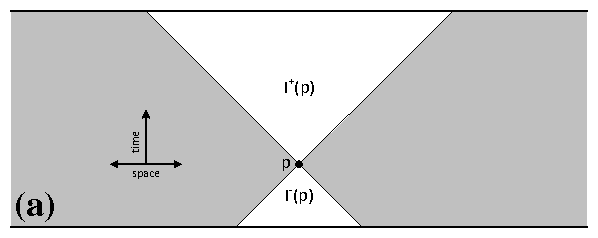
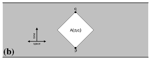
For each point p on a Lorentzian manifold M, one can split the set of all points at timelike distances from p into two parts: I⁻(p)-all points in the past of p whose time coordinate is smaller than p's, and I⁺(p)-all points to the future of p, see Fig. 2(a). If point q ∈ I⁺(p), then intersection A(p,q)=I⁻(q)∩I⁺(p) is called an Alexandrov set, see Fig. 2(b). These sets form a base of a topology on M called the Alexandrov topology. Manifold M is called strongly causal if there are no closed timelike curves on M, and if there is no point p ∈ M with timelike curves passing via its small neighborhood (see e.g. [10] for formal definitions and further background). If M is strongly causal, which is the case for all the manifolds we will consider in this project, then the Alexandrov topology on M agrees with its standard manifold topology [11]. Informally, this fact means that Alexandrov sets are analogs of open balls in the Riemannian case. In view of the definition of random hyperbolic graphs in Section 4.2, this analogy leads us to a natural definition of random Lorentzian graphs.

Figure 2: Lorentzian geometry. The grey color shows a subset of a Lorentzian manifold with the value of the time coordinate lying in a certain range. The white color in panel (a) shows the sets of points I⁻(p) and I⁺(p) at negative distances from point p in its past and future. The white color in panel (b) shows the Alexandrov set A(p,q)=I⁻(q)∩I⁺(p) of two points p and q. Panel (c) shows a finite point set, in which all pairs of points at negative distances are connected, thus forming a graph. In this graph, if two points p and q are connected, then A(p,q) contains all their common neighbors. If the graph is an RLG, then the number of common neighbors connected to two connected nodes p and q is a random variable distributed according to the Poisson distribution with the mean equal to the volume of A(p,q).

4.4 Random Lorentzian Graphs (RLGs)

In analogy with RHGs, we propose to constructively define random Lorentzian graphs (RLGs) as follows:

consider a compact subset (patch) P of Lorentzian manifold M;
distribute N nodes on P with a uniform node density, e.g., by the Poisson point process; and
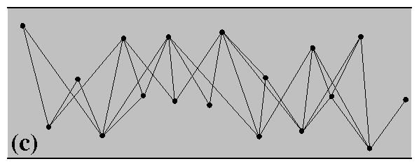
connect all pairs of nodes located at timelike distances, see Fig. 2(c).

The fact that Alexandrov sets in Lorentzian geometry are analogous to open balls in Riemannian geometry justifies the last point in the definition.

The main deliverables of Task 1 in Section 3 are manifold M and patch P whose RLGs model real networks, as well as the proof that P is invariant under the group of isometries of M. In what follows we describe the most likely candidates for M and P.

An important feature of the RHG model is its simplicity. The simplest formulation of the model uses the simplest hyperbolic manifold, i.e., the hyperbolic plane, and the simplest compact patch in it, i.e., a hyperbolic disc, invariant under the group of hyperbolic isometries SO(1,2). To identify M and P we will use a similar strategy, starting with the simplest Lorentzian manifolds and their compact subsets.

The simplest Lorentzian manifolds are Lorentzian manifolds with constant curvature, which can be zero, positive, or negative. The corresponding spaces are called Minkowski, de Sitter, and anti-de Sitter spaces. In two dimensions, their metrics in the "polar" coordinates are:

ds²

−dt² + dr², t ∈ (−∞,∞), r ∈ (−∞,∞),

(6)

ds²

−dt² + cosh²t dr², t ∈ (−∞,∞), r ∈ [0,2π),

(7)

ds²

−cosh²r dt² + dr², t ∈ [0,2π), r ∈ (−∞,∞),

(8)

and their groups of orientation-preserving isometries are SO(1,1), SO(1,2), and SO(2,1). In the above expressions, t is the time coordinate, and r is the space "radial" coordinate. In the Minkowski space, one can immediately see that sets of points at zero distances from any point p, forming the boundaries of I⁻(p) and I⁺(p), lie on straight lines intersecting the t- and r-axes at 45^o (Fig. 2). In the de Sitter space, the spatial coordinate r ∈ [0,2π) spans a circle, so does time t ∈ [0,2π) in the anti-de Sitter space, thus forming closed timelike curves. Yet in the latter case one can unwrap time to be t ∈ (−∞,∞) by considering the universal cover of the space, which does not have closed timelike curves. Both de Sitter and anti-de Sitter spaces can be represented as one-sheeted hyperboloids in the three-dimensional Minkowski space. Coordinates lines of constant r and, respectively, t are hyperbolas on these hyperboloids.

Direct inspection of Eqs. (6-8) and (1) suggests that the de Sitter space is the most likely candidate for M. Indeed, space (circles) expands exponentially with time t in this space, similarly to its exponential expansion with r in the hyperbolic plane-the key property yielding power-law degree distribution in RHGs. In the Minkowski space, there is no exponential expansion, while in the anti-de Sitter space, not space but time expands exponentially with r. Further, the group of isometries of the d-dimensional de Sitter space is the same as the group of hyperbolic isometries, SO(1,d), vs. SO(2,d−1) for anti-de Sitter space-yet another indication that out of these three simplest Lorentzian manifolds, the de Sitter space is the most likely candidate.

Focusing on de Sitter space for a moment, we show that a particular definition of RLGs on it leads to power-law graphs with exponent γ = 2. To define RLGs, we have to fix patch P first. The coordinate system in Eq. (7), in view of its similarity to Eq. (1), dictates to define patch P as a compact subset lying between t=0 and t=τ, mimicking hyperbolic discs, which are compact subsets of H lying between r=0 and r=R, except that τ is now a dynamical variable modeling graph growth with time. With this choice, a particular ensemble of RLGs is now fully defined. Equation (7) leads to the following temporal node density:

ρ(t)=

cosht

sinhτ

≈ e^t−τ, where t ∈ [0,τ],

(9)

similar to Eq. (3).

Consider now node p at time coordinate t ∈ [0,τ]. Since nodes are distributed uniformly in P, p's degree is proportional to the sum of areas I⁺(p) and I⁻(p) (Fig. 2). To compute these areas we have two options: either derive the equations for the boundaries of I⁺(p) and I⁻(p) in the (t,r) coordinates, or change the time coordinate t to conformal time coordinate η defined by dη = dt/cosht, i.e., secη = cosht, η ∈ (−π/2,π/2). In these coordinates the metric in Eq. (7) and the volume form on patch P become

ds²

sec²η(−dη² + dr²), η ∈ [0,arcseccoshτ], r ∈ [0,2π),

(10)

sec²η dη dr,

(11)

and the boundaries of I⁺(p) and I⁻(p) are straight lines intersecting the η- and r-axes at 45^o. Therefore, with notations η_t=arcseccosht and η_T=arcseccoshτ, the areas |I⁺(p)| and |I⁻(p)| are given by

|I⁺(p)|

⌠
⌡

η_T

η_t

dη′

⌠
⌡

η′−η_t

0

dr sec²η′=ln

cosη_T

cosη_t

+(η_T−η_t)tanη_T,

(12)

|I⁻(p)|

⌠
⌡

η_t

0

dη′

⌠
⌡

η_t−η′

0

dr sec²η′=lnsecη_t=lncosht.

(13)

For large times t >> 0, the second integral is simply proportional to t, while if τ >> t >> 0, then the first integral, and consequently the expected degree k(t) of node p at time coordinate t, scale as

|I⁺(p)| ∼ k(t) ∼ e^τ−t.

(14)

That is, similar to RHGs, we observe the combination of two exponentials, the density of nodes in Eq. (9) and their expected degrees in Eq. (14). Yet we notice an important difference between Eqs. (5) and (14): the exponent in the latter is not 1/2 but 1, yielding the power-law degree distribution in RLGs with exponent γ = 1+1=2.

We may find however that map Φ described in Task 1 does not exist, or that it is not extensible for higher dimensions, or that it is not invariant under SO(1,d), in which case the RLG construction above, contrary to RHGs, is just an artifact of a particular choice of the coordinate system and patch P. That is, such RLGs do not really reflect the geometry of the underlying manifold. If none of the Lorentzian spaces with constant curvature satisfy the requirements of Task 1, then we will consider a wider class of homogeneous and isotropic Lorentzian manifolds whose metric can be written as

ds²=−dt²+a²(t)dΩ²,

(15)

where the spatial part of the metric dΩ does not depend on time. An even wider class of manifolds are manifolds with only spherical symmetry with metric

ds²=−dt²+a²(t,r)dΩ²,

(16)

where r is the radial coordinate. We expect that manifold M representing real networks will belong to this class since RHGs must be dual, in the sense of Task 1, to RLGs, and since the RHG definition is manifestly spherically symmetric.

Task 1 is the most intellectually challenging. The other tasks described in Section 3 are work-intensive as well. To accomplish these tasks we will use the methods and results from our previous work [2,3,4,5,6,7,8], described in Sections 4.1-4.2. We emphasize that the graphs we will consider, both real networks and synthetic RLGs, will be dynamic. That is, we will collect detailed historical data on networks that evolve in time, vs. their one-time snapshots, and juxtapose their structural and dynamics properties against those in RLGs. The growth dynamics of RLGs will be modeled by parameter τ (or its equivalent). As τ grows by dτ, nodes p with time coordinates in the interval [τ,τ+dτ] join anew an RLG existing by time τ, and connect to all the existing nodes lying in I⁻(p).

4.5 Impact and significance

A successful outcome of this project will constitute a significant step forward towards a conceptually different set of tools for anomaly detection in real networks. In shorter term, it will likely increase the prediction accuracy of the large-scale dynamics of complex networks. Indeed, if a network grows exactly as an RLG, then the probability of the existence of a (new) link between a pair of nodes is either 1 or 0, depending on whether the Lorentzian distance between two nodes is negative or positive. That is, in this hypothetical case, the link prediction accuracy reaches 100%! However, real networks are stochastic dynamical systems, whose measurement is prone to errors and noise. This stochasticity, inevitably present in real networks, prevents the prediction accuracy from reaching 100%. Note that the temperature parameter in our geometric model in Section 4.2 is a base-line parameter modeling noise and fluctuations in the network. At zero temperature, the ties between network structure and underlying geometry are strongest, and the duality between RHGs and RLGs given by Φ is exact. At higher temperatures characterizing real networks, these ties weaken, and the equivalence can no longer be exact. Since the values of temperature characterizing real networks are close to zero [7], the deviations from the exact case cannot be strong, but nevertheless we will quantify their effect on the prediction accuracy in Task 5.

4.6 Future work

The work proposed above for the first year is by no means our final goal. A successful outcome of this project will prove that RLGs describe the structure and dynamics of real networks at the large scale. The manifolds M from Task 1 will likely be homogenous and isotropic, as is the hyperbolic space in RHGs. If we take a real network, however, e.g., the real Internet, and map it to its homogeneous hyperbolic space, we observe that after the mapping, the node density in H deviates strongly from uniform [7]. This observation naturally suggests that in reality the latent space is homogenous only at the largest scale, while at smaller scales there are some inhomogeneities and anisotropies. In our future work we will have to account for these deviations. Without doing so, we will not be able to derive the universal laws of network dynamics at smaller scales, and to describe fine-grained dynamics of these networks.

If successful, this future task will establish the universal laws of fine-grained dynamics of nodes and links in complex networks, leading to new powerful methods and tools in network analysis, prediction, and anomaly detection. Indeed, we will be able to predict not only the large-scale dynamics of network growth, but also node trajectories in the latent space, the probability of the appearance of new nodes in a given area of this space in evolving networks, etc. More importantly, knowing the node trajectories, we will be able to predict fine-grained dynamics of edge appearances and disappearances, simply because these edges exist or do not exist depending on whether the Lorentzian distances between corresponding nodes are negative or positive. Deviations from this dynamics will then indicate anomalous activity, which we can distinguish from noise and fluctuations as discussed in Section 4.5.

To this end, we will also have to learn the dimension of Lorentzian manifolds underlying real networks, using persistent homology or other methods. If this dimension turns out to be larger than 2, then we will also have to improve the network mapping methods developed in [7]. To infer latent geometric coordinates of nodes in real networks, these methods utilize Markov Chain Monte Carlo (MCMC) algorithms-specifically, the Metropolis-Hastings algorithm [14]-which scale poorly with network size. In fact, they do not provide any computation complexity guarantees. Moreover, substantial manual intervention and guidance are required to aid those algorithms to converge and produce reliable results. Moving from two dimensions as in [7] to higher dimension d > 2 which may characterize some real network datasets, will require inferring few times as many hidden variables for each node-d−1 spatial coordinates instead of one. It seems unlikely that MCMC algorithms will scale for any reasonably-sized real network in this case. Therefore another research direction in our future work is to develop optimal methods to infer latent spatial node coordinates in large real networks.

5 Comparison with Other Ongoing Research

The most widely used approaches to anomaly detection and network dynamics prediction are based on data mining, machine learning, and statistics. These approaches can be very useful in certain cases, yet their limitations are well known. These approaches lack universality: they are often highly tailored to a specific network or specific task, leading to overfitting, overtraining a method on a specific dataset, and thus diminishing the predictive power of the method and its overall efficiency. Worse yet, extreme manual care and special expertise are routinely required to tune these approaches for a task at hand, rendering them nearly impossible to use in everyday practice with constantly changing requirements and conditions.

In this project we strive to develop a radically different approach. Our goal is to discover the universal laws governing the dynamics of complex networks, since the knowledge of such laws will allow us to predict network dynamics, while abnormal dynamics deviating from such laws will then signify anomalous activity in the network. Based on the results from our previous work, we argue in the project description above that such laws can be derived within the theory of random geometric graphs.

Random graphs in general and random geometric graphs in particular form a vast and intensively studied area of research in mathematics. The most popular and best studied graph models include classical (Erdös-Rényi) random graphs [15], random graphs with a given (expected) degree distribution [16], and random geometric graphs in Euclidean spaces [17], which we review next.

Perhaps the simplest random graph ensemble is the G_N,p ensemble of classical random graphs, defined as random graphs of N nodes in which each pair of nodes is independently connected with probability p. Structurally, these random graphs are very different from real networks, since the degree distribution in these random graphs is Poissonian, and clustering is asymptotically zero, versus fat-tailed degree distribution and strong size-independent clustering in real networks [1].

Random graphs with a given expected (power-law) degree distribution simply enforce the degree distribution in random graphs to any pre-defined shape using the following constructive definition. Given a set of N nodes, and any desirable distribution ρ(κ) of expected degrees κ, construct the graph by first assigning to each node i=1,…,N a random variable κ_i independently drawn from distribution ρ(κ), and then connection each pair of nodes i and j with probability p_ij ∼ κ_i κ_j. One can then show that under certain conditions, the degree distribution in thus-defined graphs is well approximated by ρ(κ). If one takes ρ(κ) to be a power law, then these random graphs have a power-law degree distribution, but clustering is still asymptotically zero.

Random geometric graphs in Euclidean spaces have found many important applications, especially in the theory and practice of wireless networks [18]. In the simplest case, these graphs are defined by the following construction. Consider a compact patch P of a Euclidean space, e.g., a unit square in the Euclidean plane, distribute N nodes over P uniformly at random, e.g., using the Poisson point process, and finally connect each pair of nodes iff the Euclidean distance between them does not exceed a certain threshold R. Since these graphs are geometric, they have strong clustering-similar to RHGs, the large number of triangular subgraphs in these graphs is a consequence of the triangle inequality in the underlying space-but their degree distribution is Poissonian, as in the classical random graphs.

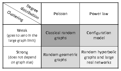
In summary (see Table 1), none of these random graph models describe properly all the common structural properties of real networks. The main contribution of our previous work described in Section 4 is the proof that random geometric graphs in hyperbolic spaces fill this gap. Yet this graph model has its own limitations, which we set to resolve in this project. If successful, this project will result in a graph model, describing better real networks, and moving us a step closer to being able to predict the dynamics of these networks, and detect anomalous activity in them.

Table 1: Taxonomy of random graphs and their basic structural properties

6 Our Previous Accomplishments in Related Areas

Another area of our research, not mentioned in Section 4, deals with detailed analysis of real network data, especially that of the Internet. Among many results in that area, the works that were cited more than 100 times according to Google Scholar include the analysis of the statistical properties of the Internet [19], inference of business relationships between autonomous systems [20], development of a systematic series of degree-based statistics for network analysis and generation (dK-series) that was later used in graphlets [21], and applications of compact routing to Internet(-like) graphs [22,23].

References

[1]: M E J Newman. The Structure and Function of Complex Networks. SIAM Rev, 45(2):167-256, 2003. http://dx.doi.org/10.1137/S003614450342480.
[2]: M. AÌngeles Serrano, Dmitri Krioukov, and Marián Boguñá. Self-Similarity of Complex Networks and Hidden Metric Spaces. Phys Rev Lett, 100:78701, 2008. http://dx.doi.org/10.1103/PhysRevLett.100.078701.
[3]: Marián Boguñá, Dmitri Krioukov, and Kc Claffy. Navigability of Complex Networks. Nature Physics, 5:74-80, 2009. http://dx.doi.org/10.1038/NPHYS1130.
[4]: Marián Boguñá and Dmitri Krioukov. Navigating Ultrasmall Worlds in Ultrashort Time. Phys Rev Lett, 102:58701, 2009. http://dx.doi.org/10.1103/PhysRevLett.102.058701.
[5]: Dmitri Krioukov, Fragkiskos Papadopoulos, Amin Vahdat, and Marián Boguñá. Curvature and Temperature of Complex Networks. Phys Rev E, 80:035101(R), 2009. http://dx.doi.org/10.1103/PhysRevE.80.035101.
[6]: Dmitri Krioukov, Fragkiskos Papadopoulos, Maksim Kitsak, Amin Vahdat, and Marián Boguñá. Hyperbolic Geometry of Complex Networks. Phys Rev E, 82:36106, 2010. http://dx.doi.org/10.1103/PhysRevE.82.036106.
[7]: Marián Boguñá, Fragkiskos Papadopoulos, and Dmitri Krioukov. Sustaining the Internet with Hyperbolic Mapping. Nature Comms, 1:62, 2010. http://dx.doi.org/10.1038/ncomms1063.
[8]: M. AÌngeles Serrano, Dmitri Krioukov, and Marián Boguñá. Percolation in Self-Similar Networks. Phys Rev Lett, 106(4):048701, January 2011. http://dx.doi.org/10.1103/PhysRevLett.106.048701.
[9]: Misha Gromov. Metric Structures for Riemannian and Non-Riemannian Spaces. Birkhäuser, Boston, 2007.
[10]: John K. Beem, Paul Ehrlich, and Kevin Easley. Global Lorentzian Geometry. CRC Press, New York, 1996.
[11]: A. D. Alexandrov. Filosofskoe Soderzhanie i Znachenie Teorii Otnositel'nosti. Voprosy Filosofii, 1:67-84, 1959.
[12]: Leslie G. Valiant. Circuits of the Mind. Oxford University Press, New York, 1994.
[13]: J Park and M E J Newman. Statistical Mechanics of Networks. Phys Rev E, 70:66117, 2004. .
[14]: M E J Newman and G T Barkema. Monte Carlo Methods in Statistical Physics. Clarendon Press, Oxford, 1999.
[15]: P Erdös and A Rényi. On Random Graphs. Publ Math, 6:290-297, 1959.
[16]: F Chung and L Lu. The Average Distance in a Random Graph with Given Expected Degrees. Internet Math, 1(1):91-114, 2003.
[17]: M Penrose. Random Geometric Graphs. Oxford University Press, Oxford, 2003.
[18]: M Franceschetti and R Meester. Random Networks for Communication: From Statistical Physics to Information Systems. Cambridge University Press, Cambridge, 2008.
[19]: Pria Mahadevan, Dmitri Krioukov, Marina Fomenkov, Bradley Huffaker, Xenofontas Dimitropoulos, Kc Claffy, and Amin Vahdat. The Internet AS-Level Topology: Three Data Sources and One Definitive Metric. Comput Commun Rev, 36(1):17-26, 2006. http://dx.doi.org/10.1145/1111322.1111328.
[20]: Xenofontas Dimitropoulos, Dmitri Krioukov, Marina Fomenkov, Bradley Huffaker, Young Hyun, Kc Claffy, and George Riley. AS Relationships: Inference and Validation. Comput Commun Rev, 37(1):29-40, 2007. http://dx.doi.org/10.1145/1198255.1198259.
[21]: Pria Mahadevan, Dmitri Krioukov, Kevin Fall, and Amin Vahdat. Systematic Topology Analysis and Generation Using Degree Correlations. In SIGCOMM, 2006. http://dx.doi.org/10.1145/1151659.1159930.
[22]: Dmitri Krioukov, Kevn Fall, and Xiaowei Yang. Compact Routing on Internet-Like Graphs. In INFOCOM, 2004. http://dx.doi.org/10.1109/INFCOM.2004.1354495.
[23]: Dmitri Krioukov, Kc Claffy, Kevin Fall, and Arthur Brady. On Compact Routing for the Internet. Comput Commun Rev, 37(3):41-52, 2007. http://dx.doi.org/10.1145/1273445.1273450.

File translated from T_{EX by T_TH, version 3.87.

On 4 Jan 2013, 15:17.}